Over the past months the EIS Analyzer has evolved from a Streamlit prototype into a full-featured native application. This article summarizes the most significant improvements across the 2.0, 2.1 and 2.2 release series — focused on trustworthy results, less manual tuning, and faster batch workflows.

The Batalyse EIS Analyzer is a desktop application for analyzing Electrochemical Impedance Spectroscopy (EIS) data from batteries, fuel cells, supercapacitors and electrochemical sensors. It supports the major instrument file formats (Bio-Logic, Gamry, Solartron, PalmSens, Zahner) and provides a complete workflow from raw data import through equivalent-circuit fitting, Distribution of Relaxation Times (DRT) analysis, Kramers-Kronig validation and feature extraction to Origin (.opju) and CSV export. It is developed by Batalyse GmbH and is part of the broader Batalyse Collect platform for battery R&D data management.

All upgrades are driven by user feedback and a thorough audit against established literature in electrochemical impedance analysis.

A new architecture (2.0)

The foundation was rebuilt from the ground up: a FastAPI backend paired with a TypeScript frontend, delivered as a native desktop application via pywebview with browser fallback. Alongside this came a suite of major analysis features that shape today’s workflow:

• DRT analysis with automatic equivalent-circuit recommendation [1]
• Auto-Analysis pipeline chaining DRT, fitting, K-K validation and feature extraction in one click, with trend analysis across loaded files
• SOH and temperature estimation from extracted EIS features
• Origin (.opju) export with multi-sheet workbooks for downstream analysis in OriginLab
• Project import/export (.batalyse files) for reproducible session sharing
• SQL connectivity (MySQL and SQL Server) for direct database integration
• PalmSens .pssession support, in addition to Gamry, Bio-Logic and Solartron formats
• Graph customization with a preset library for consistent publication-quality figures
• Automatic update checking with rollback support

Transmission Line Models and constrained fitting (2.1)

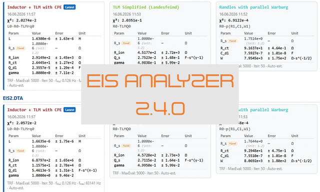
For porous electrodes — battery cathodes, supercapacitors, fuel cell catalyst layers — equivalent circuits with lumped elements often miss the distributed nature of the impedance response. Release 2.1 added a complete suite of Transmission Line Models (TLM) based on de Levie’s framework [2]: blocking, R||C, R||CPE, RC + Warburg, transmissive variants, and nested (hierarchical) macro/meso models for multi-scale porous architectures.

The same release introduced constrained fitting through lmfit: parameters can now be fixed, bounded, or linked to other parameters via mathematical expressions. The constraint engine integrates seamlessly with the optimizer and supports per-parameter tightened bounds appropriate to the parameter type (CPE exponents [0.3, 1.0], inductors [10⁻¹², 10⁻³] H, etc.).

A multi-language interface (9 languages) and visual frequency-range selection by clicking on the Bode/Nyquist plot completed this release.

Scientifically validated fitting improvements (2.2)

The auto-estimate engine now leverages Distribution of Relaxation Times (DRT) to derive initial parameter values directly from the spectrum’s time-constant fingerprint — an approach widely recognized in the EIS literature for improving the convergence of complex nonlinear least-squares fits [1, 3]. For each RQ element, peak τ values from the DRT are converted into accurate R and Q estimates via the relation Q = τⁿ/R, far more reliable than heuristic peak detection in spectra dominated by diffusion tails.

For complex spectra without resolvable semicircles, capacitance is now estimated using the half-circle frequency method [4] — finding the frequency where Z’ equals R_s + R_ct/2 — instead of the previous argmax(−Z”) approach that failed on monotonic spectra. This single change improved auto-estimate accuracy by orders of magnitude on diffusion-dominated battery impedance data.

To escape local minima, a multi-start optimization strategy [5] automatically retries the fit with perturbed initial guesses when χ² remains above 10⁻². Studies of EIS fitting workflows have shown such pre-fit strategies can raise Randles-circuit fitting success rates from approximately 50% to over 97% [5].

Unified Kramers-Kronig quality scoring (2.2)

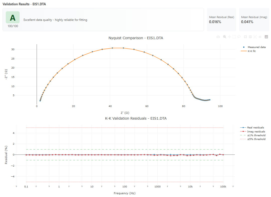
The K-K validation [6, 7] previously suffered from three independent quality-score implementations that could disagree — a user could see “Grade A” alongside “K-K Validation Failed.” This has been replaced with a single source of truth. Pass/fail, numerical score, and letter grade are now derived from the same statistics with identical thresholds. Grade A or B always means valid; an invalid verdict can never coexist with a top grade.

Unified parameter table with shared-parameter fitting (2.2)

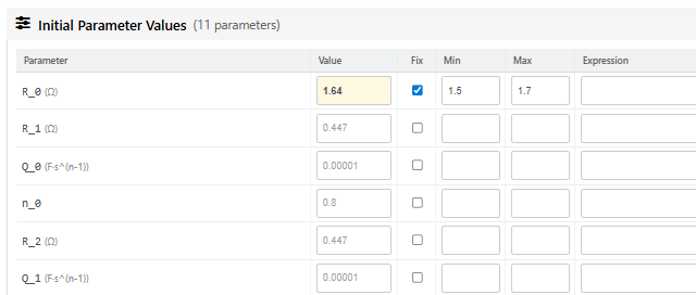
The redesigned Fitting tab merges what were previously two separate sections — Initial Parameter Values and Advanced Constraints — into a single intuitive table with columns for Parameter, Value, Fix, Shared, Min, Max, and Expression.

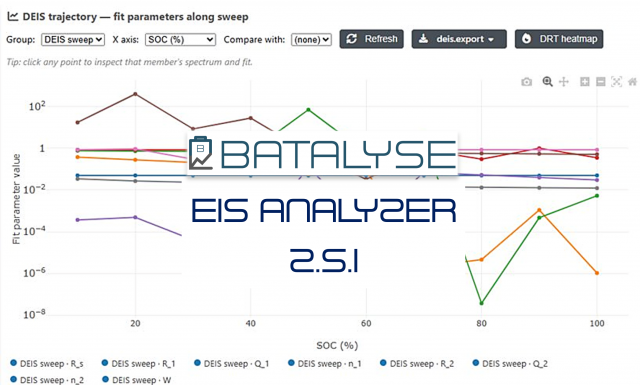
Each column has a hover tooltip explaining its effect. The new Shared column enables true global parameter linking: when one or more parameters are marked as shared and multiple sweeps or files are loaded, those parameters are fit as a single value across every sweep of every file simultaneously — a workflow essential for tracking the series resistance R_s of one cell across many state-of-charge points without artificial drift.

Fitting tab sees what the Plots tab sees (2.2)

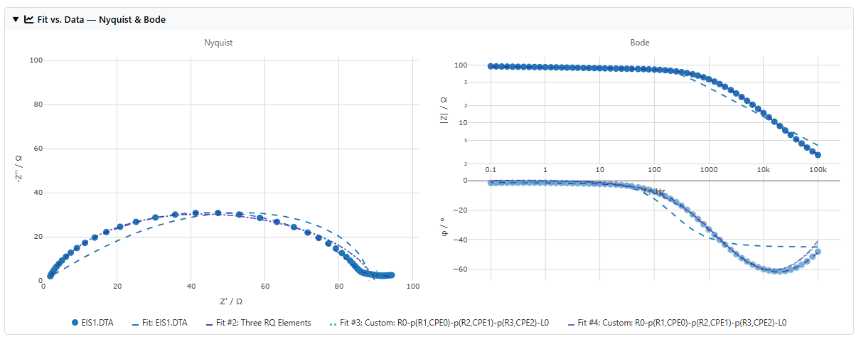
The Fitting tab’s “Fit vs. Data” section now shows all sweeps with their fits and full fit history, color-matched to the main Plots tab. The active sweep is highlighted with larger markers and full opacity; previous fit attempts appear as dashed history lines for visual comparison. Clicking a legend item toggles the corresponding curves in both compact and main plots simultaneously.

Smarter UI guidance (2.2)

When a fit converges with mediocre quality but R_s is well-determined (relative error < 10%), the app now suggests fixing R_s with one click — a standard EIS workflow recommendation [8]. A blue tip appears below the fit result with a “Fix R_s = X Ω” button that updates the input and checks the Fix box automatically.

References

[1] Wan, T. H., Saccoccio, M., Chen, C., Ciucci, F. Influence of the discretization methods on the distribution of relaxation times deconvolution: implementing radial basis functions with DRTtools. Electrochimica Acta 184 (2015) 483–499. doi:10.1016/j.electacta.2015.09.097

[2] de Levie, R. On porous electrodes in electrolyte solutions — IV. Electrochimica Acta 9 (1964) 1231–1245. doi:10.1016/0013-4686(64)85015-5

[3] Heinzmann, M., Weber, A., Ivers-Tiffée, E. Advanced impedance study of polymer electrolyte membrane single cells by means of distribution of relaxation times. Journal of Power Sources 402 (2018) 24–33. doi:10.1016/j.jpowsour.2018.09.004

[4] Hsu, C. H., Mansfeld, F. Technical note: Concerning the conversion of the constant phase element parameter Y₀ into a capacitance. Corrosion 57 (2001) 747–748. doi:10.5006/1.3280607

[5] Pfeiffer, K., Ulm, L., Wachter, A., Dempwolf, S., Pretzler, M., Rompel, A., Heuberger, A. Impact of normalization, standardization and pre-fit on the success rate of fitting in electrochemical impedance spectroscopy. Current Directions in Biomedical Engineering 7 (2021) 488–491. doi:10.1515/cdbme-2021-2125

[6] Boukamp, B. A. A linear Kronig-Kramers transform test for immittance data validation. Journal of the Electrochemical Society 142 (1995) 1885–1894. doi:10.1149/1.2044210

[7] Schönleber, M., Klotz, D., Ivers-Tiffée, E. A method for improving the robustness of linear Kramers-Kronig validity tests. Electrochimica Acta 131 (2014) 20–27. doi:10.1016/j.electacta.2014.01.034

[8] Lazanas, A. C., Prodromidis, M. I. Electrochemical impedance spectroscopy — A tutorial. ACS Measurement Science Au 3 (2023) 162–193. doi:10.1021/acsmeasuresciau.2c00070